The transformer is a learned probability model

Helloo,

Transformer is the model architecture used by Large Language Models. It was introduced by the Google Brain team in 2017 in the famous research paper — “Attention is all you need”.

The latest trillion parameter models trained by frontier labs, that feel like magic, out of a science fiction book, are scaled up versions of this architecture. There have been a few tweaks to the architecture over the years but the core is still the same.

In this blog we’ll go over high level Math behind the transformer architecture. Let’s Go!

Transformers are from the class of autoregressive models. Which means you generate tokens one by one. Each new token depends on the previous tokens.

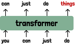
The first step is, to convert raw input text into tokens. This step is called Tokenization. It is the process of breaking down Raw Text into chunks.

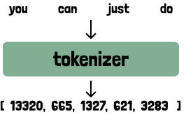
There are multiple ways to build the Tokenizer algorithm. It could be as simple as tokenizing on characters, tokenizing on whitespaces (words), but currently the most widely used technique is BPE Tokenizer. Check out Andrej Karpathy’s video on Tokenization for a deep dive. We are moving forward, as this step is comparatively trivial and we have a lot to cover.

The token is the smallest unit a model sees. Tokens have a fixed vocabulary size $V$. Current state of the art models (GPT-5, Opus) have a vocab size of 100K-200K tokens.

When we say training a model, it means learning the underlying probability distribution of the sequence of tokens. This sequence of tokens can be anything — code, essays, images, music…

And then inference simply becomes sampling from this learned probability distribution given a sequence of input tokens.

The question is how do we make the model learn this probability distribution?

If $P^*$ is the real world probability distribution of human generated text. We have to learn a model that approximates human text generation. We’ll call this $P_\theta$

If we have 3 human generated sentences —

1. the cat sat on the mat
2. the cat sat zx oj squid
3. Paris is the capital of France

In real world the probability of seeing a sentence like 2 is near zero, no human will write like that. So $P^*$ will give it near 0 prob. and we expect $P_\theta$ to do the same.

$P^*$ can be defined as

$$P^* = P(x_1, x_2, \dots, x_T)$$

where $P(x_1, x_2, \dots, x_T)$ is the joint probability over the sequence of input tokens of length $T$. What we’re saying is — I want to know the probability of seeing a particular sequence $(x_1, x_2, \dots, x_T)$. On each position I have $V$ options, so for the sequence of length $T$ the number of options to choose from becomes $V^T$

The naive way to learn this joint probability is:

1. Build a giant lookup table: one row for every possible sequence of length $T$, which is $V^T$ rows. Where we store the occurrence of each sequence, count how often each appears and normalize to get probabilities. This approach is not feasible.
   1. Even with a moderate size of $V = 50000$ vocab and just $T = 100$ sequence length. Since we can have 50000 choices at each position the size of the table becomes $50000^{100}$ which is larger than the number of atoms in the universe. And the $T = 100$ sequence length is nothing compared to real world sequences.
   2. Second, if this model sees a sequence it has not seen before it will assign it a score of zero. This table will be incredibly sparse.

We tackle this problem by using the chain rule.

The chain rule states that the joint probability of a sequence of events can be expressed as the product of conditional probabilities of each event, given the events that came before it.

Mathematically, it can be expressed as:

$$\begin{aligned} P^* &= P(x_1, x_2, \dots, x_T) \\ &= P(x_1) \cdot P(x_2 \mid x_1) \cdot P(x_3 \mid x_1, x_2) \\ &\quad \cdots P(x_T \mid x_1, x_2, \dots, x_{T-1}) \end{aligned}$$

This is amazing. The joint probability $P(x_1, x_2, \dots, x_T)$, which was impossible to compute, now breaks into $T$ smaller problems that all look exactly the same — given the tokens so far, what is the next token?

Each of these smaller problems is a function. It takes the previous sequence as input, and outputs a probability distribution over the next token. That distribution is always a vector of size $V$, one probability for every token in the vocabulary, no matter how long the input sequence is. And we don’t memorize a $50000^{100}$ lookup anymore — we learn the weights of this one function, and the same weights serve every position and every sequence length.

Let’s call this function $P_\theta$, where $\theta$ are the learned weights.

$$P_\theta(\text{next token} \mid \text{previous sequence})$$

And we can stack this up. $P_\theta$ gives us a distribution over the next token, we pick a token from it, append it to the sequence, and call $P_\theta$ again on the longer sequence to get the token after that. Keep going till we reach the end of the sequence. Multiply the $P_\theta$’s along the way and we get back the probability of the whole sequence.

The transformer is this function $P_\theta$ — given an input sequence, it predicts the probability distribution of the next token. Training a transformer means learning the weights $\theta$.

One small note on notation before we go further. To keep every step uniform we add a special start token $x_0$ at the front of the sequence. This way even the very first token is a conditional — $P(x_1)$ is really $P(x_1 \mid x_0)$ — and every step looks the same.

Let’s see how this unfolds.

So after converting, raw text —> tokens

Each token is represented by a numerical id in a fixed vocabulary. Each token is depicted by a vector of raw numbers called embedding. The embedding encodes the semantic meaning of the token in a numerical format. You can imagine it being like a dictionary of token_id and embedding vector —

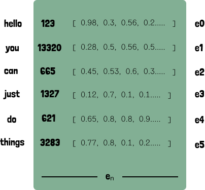
We’ll denote embedding vectors by $e_t$

The tokens are converted into embeddings, which we get by just a lookup in the embedding matrix. The embedding matrix is learned at training time and fixed during inference.

Here is what each symbol in the diagram means —

$x_t$ — the token at position $t$. The input sequence is $X = (x_0, x_1, \dots, x_{T-1})$

$e_t$ — the embedding vector of $x_t$. This is what actually goes into the transformer, the transformer never sees the raw token id.

$u_t$ — the output at position $t$. Before we can say what’s in it, we need a name for the tokens in the vocabulary. The vocabulary is a fixed list of $V$ tokens, we’ll call them $v_1, v_2, \dots, v_V$. Now, $u_t$ is a vector of $V$ raw scores, one for each vocabulary token. The $k$-th entry is a score for how likely $v_k$ is to be the next token $x_t$, given everything that came before it, $x_0, x_1, \dots, x_{t-1}$. Higher score means more likely. These raw scores are called logits.

There is one $u$ vector at every position. $u_1$ sits above $x_0$ and scores what comes after $x_0$. $u_2$ sits above $x_1$ and scores what comes after $x_0, x_1$. And so on. That’s why in the diagram the $x$’s start at 0 and the $u$’s start at 1 — $u_t$ is always the prediction for $x_t$, computed from everything before $x_t$.

We view the whole mapping from $x$’s to $u$’s as a black box in this section and call it a Transformer.

We call the transformer a function $f$ with parameters $\theta$. Given the input tokens $x_0, x_1, \dots, x_{t-1}$ it produces the logit vector $u_t$.

$$u_t = f_\theta(x_0, x_1, \dots, x_{t-1})$$

$u_t$ only depends upon $x_0, x_1, \dots, x_{t-1}$

Logits are not probabilities yet — they can be negative, and they don’t sum to 1. To turn them into a probability distribution we do a softmax over them.

It looks something like this —

$$\begin{aligned} &P_\theta(x_t \mid x_0, x_1, \dots, x_{t-1}) \\ &\qquad = \mathrm{softmax}(u_t) \\ &\qquad = \mathrm{softmax}\big(f_\theta(x_0, x_1, \dots, x_{t-1})\big) \end{aligned}$$

$f_\theta$ is the transformer, $P_\theta$ is the distribution we set out to learn. The only gap between them is the softmax — $f$ gives us the raw scores, $P_\theta$ gives us probabilities.

So the output vector has one entry per vocabulary token, where $P_\theta(x_t = v_1 \mid x_0, x_1, \dots, x_{t-1})$ is the probability of seeing $v_1$ as the next token when given the input sequence $x_0, x_1, \dots, x_{t-1}$ and so on and so forth.

Autoregressive Inference§

Given an autoregressive transformer we sample tokens from it sequentially, and the next token generated is used as an input for the next generation phase.

$$\begin{aligned} x_{t+1} &\sim \mathrm{softmax}\big(f_\theta(x_0, x_1, \dots, x_t)\big) \\ x_{t+2} &\sim \mathrm{softmax}\big(f_\theta(x_0, x_1, \dots, x_{t+1})\big) \\ &\quad\ \vdots \\ x_T &\sim \mathrm{softmax}\big(f_\theta(x_0, x_1, \dots, x_{T-1})\big) \end{aligned}$$

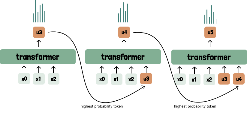
Each generated token is used as the input to the model when generating the following tokens. This is the high level math of a transformer. Keeping it as a black box.

In Part 2, we will look under the hood of a transformer and see how we get the logit vector $u$ and how each step works.